In [4]:
import locale
locale.setlocale(locale.LC_ALL, "de_AT.UTF-8");

%matplotlib inline
%precision %.4f
#%load_ext snakeviz
import colorcet
import pandas as pd
from scipy import stats
import matplotlib.pyplot as plt
import matplotlib.dates
import matplotlib.ticker
import matplotlib.patches
import matplotlib.colors
import seaborn as sns
from importlib import reload
from itertools import count
from datetime import date, datetime, timedelta
from IPython.display import display, Markdown, HTML
import textwrap
from functools import partial
from cycler import cycler
import collections

from covidat import cov, util

pd.options.display.precision = 4

cov = reload(cov)

plt.rcParams['figure.figsize'] = (16*0.7,9*0.7)
plt.rcParams['figure.dpi'] =  120 #80
plt.rcParams['figure.facecolor'] = '#fff'
sns.set_theme(style="whitegrid")
sns.set_palette('tab10')

plt.rcParams['image.cmap'] = cov.un_cmap

pd.options.display.max_rows = 120
pd.options.display.min_rows = 40
In [5]:
def stampit(fig):
    cov.stampit(fig, "Statistik Austria")
In [6]:
if False:
    st = pd.read_csv("sterbetafel-at.csv", sep=";", encoding="utf-8", header=[0,1], decimal=",", index_col=0)
    st = st.melt(ignore_index=False, var_name=["sex", "age"], value_name="life_rem")
    st.index = st.index.rename("year")
    st["age"] = st["age"].astype(int)
    st["life_sum"] = st["life_rem"] + st["age"]
    st.set_index(["sex", "age"], append=True, inplace=True)
In [7]:
def plt_sterbe_simp(st0, title):
    #sns.lineplot()
    rwidth = 1
    change = (
        st0["life_sum"]
        .groupby(level=list(set(st0.index.names) - {"year"}))
        #.transform(lambda s: s.rolling(rwidth).mean() - s.rolling(rwidth).mean().shift(rwidth))
        .transform(lambda s: s - s.shift(rwidth))
    )
    maxage = st0.index.get_level_values("age").max()
    ag60 = st0.xs(maxage, level="age")
    spread = (ag60["life_sum"] / st0.query(f"age != {maxage}")["life_sum"]).rename("exp_spread")
    #stpiv = st0.reset_index().pivot(index="year", columns="age", values="life_sum")
    #spread = (stpiv.loc[:, 60] / stpiv.loc[:, 45]).rename("exp_spread")
    #display(spread)
        #.transform(lambda s: s.rolling(rwidth).mean() - s.rolling(rwidth).mean().shift(rwidth))

    #display(spread)    #change = change[change.index.get_level_values("year") >= 1950]
    #st0 = st0[st0.index.get_level_values("year") >= 1950]
    #display(st0)
    #print(change.first_valid_index())
    #display(change[change.index.get_level_values("age") == 0].tail(12))
    plt.figure()
    ax = sns.lineplot(
        change.reset_index(), x="year", y="life_sum", hue="age", palette="Paired", marker=".",
        alpha=0.8, mew=0)
    fig = ax.figure
    fig.suptitle(
        title + (
            #f": Änderung des {rwidth}-Jahre-Schnitts ggü. {rwidth} Jahren zuvor"
            f": Änderung ggü. {rwidth} Jahren zuvor"
            if rwidth != 1 else ": Änderung ggü. Vorjahr"
        ),
        y=0.93)
    ax.legend(title="Erreichtes Alter", ncol=2)
    ax.set_ylabel("Jährliche Änderung Lebenserwartung")
    ax.set_xlabel("Jahr")
    #print(st0.iloc[0].name)
    ax.set_xlim(left=change.index[0][change.index.names.index("year")])
    #ax.axvspan(2019.5, ax.get_xlim()[1], alpha=0.5, color="yellow")
    ax.axhline(0, color="k")

    plt.figure()
    ax = sns.lineplot(
        st0.reset_index(), x="year", y="life_sum", hue="age", palette="Paired", marker=".",
        mew=0)
    ax.figure.suptitle(title, y=0.93)
    cov.labelend2(ax, st0.reset_index(), "life_sum", cats="age", x="year", shorten=lambda n: n)
    ax.set_xlim(left=st0.index.get_level_values("year")[0])
    ax.legend(title="Erreichtes Alter", ncol=2)
    ax.set_ylabel("Gesamte Lebenserwartung")
    ax.set_xlabel("Jahr")

    plt.figure()
    ax = sns.lineplot(
        spread.reset_index(), x="year", y="exp_spread", hue="age", palette="Paired", marker=".", mew=0)
    ax.figure.suptitle(title + f": Verhältnis zu {maxage}-jährigen", y=0.93)
    ax.set_xlim(left=st0.index.get_level_values("year")[0])
    ax.legend(title="Erreichtes Alter", ncol=2)
    ax.set_ylabel(f"Verhältnis Lebenserwartung zu bereits {maxage}-jährigen")
    ax.set_xlabel("Jahr")
    ax.set_ylim(bottom=1)
    cov.set_percent_opts(ax, decimals=1)
if False:
    plt_sterbe_simp(st.query("sex == 'M'"), "Österreich: Lebenserwartung Männer")
    plt_sterbe_simp(st.query("sex == 'F'"), "Österreich: Lebenserwartung Frauen")
    plt_sterbe_simp(st.groupby(level=["year", "age"]).mean(), "Österreich: Lebenserwartung Schnitt M+W")
In [10]:
bcols = ["p_die", "n_surv", "n_die", "n_at", "n_from", "life_rem"]
def mkcols(pfx): return [pfx + "_" + c for c in bcols]
cols_old = ["age"] + mkcols("m") + mkcols("f")
cols_new = cols_old + mkcols("mf")
wks = pd.read_excel(
    util.COLLECTROOT / "Jaehrliche_Sterbetafeln_1947_bis_2021_fuer_Oesterreich.ods",
    sheet_name=list(map(str, range(1947, 2002))),
    skiprows=12,
    usecols=range(len(cols_old)),
    header=None,
    names=cols_old,
    nrows=96,
    index_col=None,
)
wks.update(pd.read_excel(
     util.COLLECTROOT / "Jaehrliche_Sterbetafeln_1947_bis_2021_fuer_Oesterreich.ods",
    sheet_name=list(map(str, range(2002, 2021 + 1))),
    skiprows=7,
    usecols=range(len(cols_new)),
    header=None,
    names=cols_new,
    nrows=101,
    index_col=None,
))
In [11]:
for year, sheet in wks.items():
    sheet.dropna(inplace=True, how="all")
    sheet["year"] = int(year)
ststat = pd.concat(wks.values())
ststat["age"] = ststat["age"].astype(int)
ststat.set_index(["year", "age"], inplace=True)
ststat.columns = ststat.columns.str.split('_', n=1, expand=True)
ststat.columns.set_names(["sex", None], inplace=True)
ststat = ststat.stack(level=0)
ststat = ststat.reorder_levels(["year", "sex", "age"]).sort_index()
#lastyear = ststat.reset_index("age")["age"].groupby(["year", "sex"]).max()
ststat.loc[ststat["n_at"] == ststat["n_from"], "n_at"] = np.nan
ststat_amf = ststat.groupby(["year", "age"]).mean()
ststat_amf["sex"] = "amf"
ststat = pd.concat([
        ststat,
        ststat_amf.set_index("sex", append=True).reorder_levels(["year", "sex", "age"])
    ]).sort_index()
#display(ststat.index.dtypes)
#display(ststat_amf)
ststat["life_sum"] = ststat.index.get_level_values("age") + ststat["life_rem"]
In [12]:
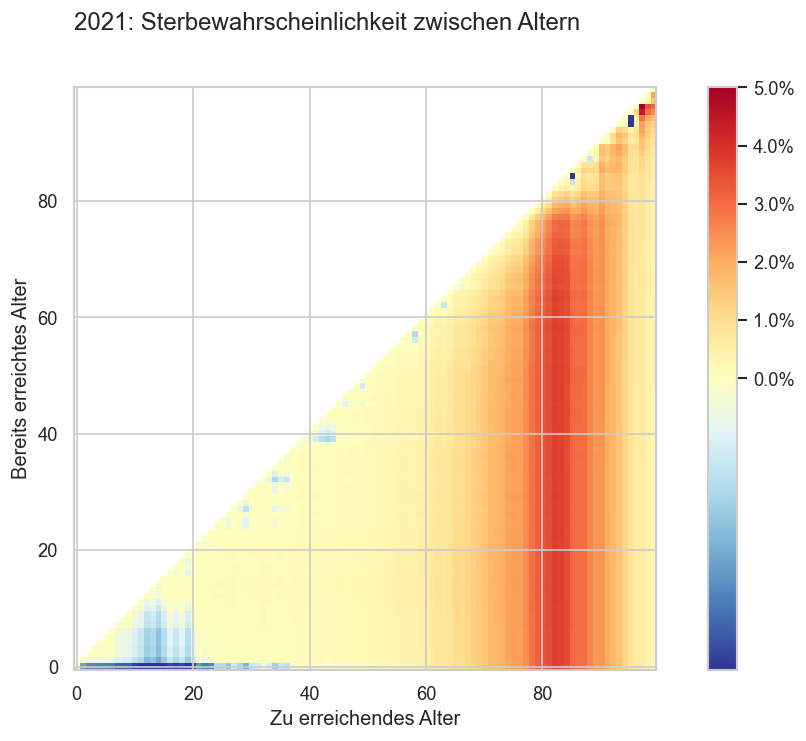
def _try_cross():
    year = 2021
    #p_surv = (1 - ststat.query("age <= 40")["p_die"]).xs((year, "m")).rename("p_surv")
    #display(n_surv)
    #p_survx = p_surv * p_surv.transpose()
    def calc_survmat(year):
        n_surv = ststat.query("age <= 99").xs((year, "m"))["n_surv"]
        survx = n_surv.to_frame().dot((1 / n_surv).to_frame().transpose())
        survx.columns = survx.columns.copy()
        survx.columns.name = "age_from"
        survx.index.name = "age_to"
        trimask = np.ones(survx.shape, dtype='bool')
        trimask[np.tril_indices(len(survx))] = False
        survx.mask(trimask, inplace=True)
        survx = survx.clip(upper=1)
        survx = (1 - survx)
        mask = np.zeros(survx.shape, dtype="bool")
        mask[np.diag_indices(len(survx))] = True
        survx[mask] = 0
        return survx
    survx = calc_survmat(year) - calc_survmat(2019)
    #display(survx)
    #survx = survx.where(lambda x: x <= 1)

    #survx = survx.sort_index(ascending=False)
    #display(survx)
    fig, ax = plt.subplots()
    vmin=0#0.0025
    #.where(lambda x: x >= vmin, vmin).mask(trimask)
    im = ax.imshow(survx.T, aspect=1, cmap=cov.div_l_cmap, interpolation='none',
                   #norm=matplotlib.colors.LogNorm(vmin=0.0025, vmax=0.05),
                   norm=matplotlib.colors.TwoSlopeNorm(vmin=-0.001, vcenter=0, vmax=0.05),
                   origin="lower")
    cax = fig.colorbar(im)
    #cov.set_logscale(cax.ax)
    cov.set_percent_opts(cax.ax, decimals=1)
    fig.suptitle(f"{year}: Sterbewahrscheinlichkeit zwischen Altern")
    ax.set_xlabel("Zu erreichendes Alter")
    ax.set_ylabel("Bereits erreichtes Alter")
_try_cross()
In [13]:
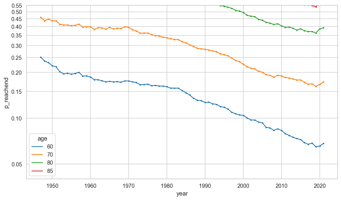
survfrom1 = (1 - ststat.query("age >= 5")["p_die"]).groupby(level=["year", "sex"]).transform(
    lambda s: s.cumprod()).rename("p_reachend")
survfrom1.xs((2019, 'f'))

def plt_surv(survdata):
    ax = sns.lineplot(
        survdata.reset_index(),
        x="year", y="p_reachend", hue="age", palette="tab10",
        marker=".", mew=0)
    cov.set_logscale(ax)
    ax.set_ylim(bottom=0.04, top=0.55)
    ax.yaxis.set_major_locator(matplotlib.ticker.MultipleLocator(0.05))

plt_surv((1 - survfrom1).reset_index().query("sex == 'amf' and age in (60, 70, 80, 85)"))
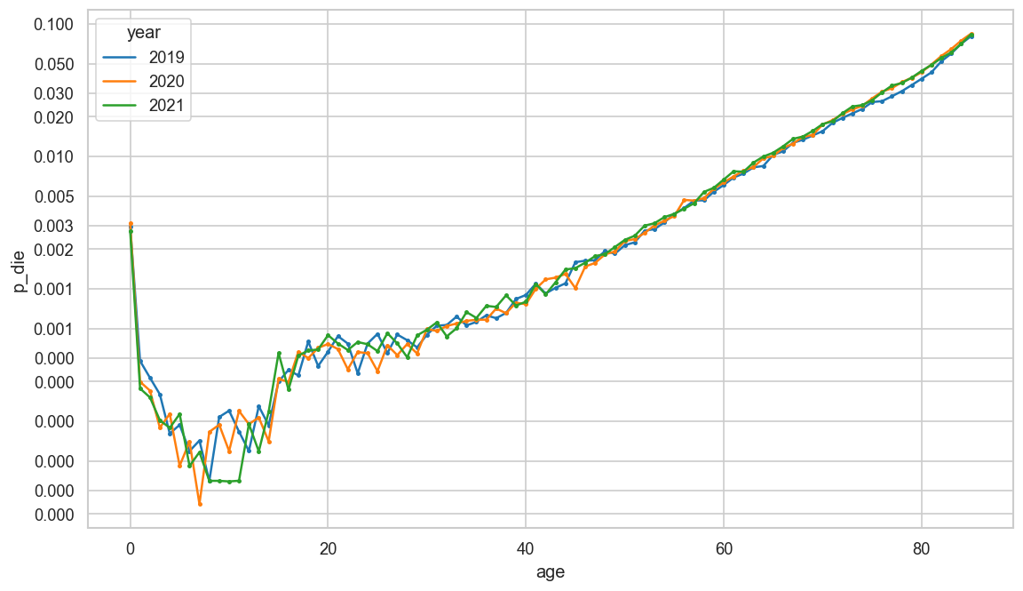
In [14]:
ax = sns.lineplot(
    ststat.reset_index()
    .query("year >= 2019 and sex == 'mf' and 0 <= age <= 85"),
    x="age",
    y="p_die",
    hue="year",
    palette="tab10",
    #markers="year",
    marker=".",
    mew=0
)
cov.set_logscale(ax)
In [15]:
if False:
    n_die5 = (1 - p_surv5) * ststat["n_surv"]
    survchange = n_die5.groupby(level=["sex", "age"]).transform(lambda s: s - s.shift().rolling(5).min())
elif False:
    n_surv5 = ststat["n_surv"]

    def lookup_maxsurv(s):
        try:
            return n_surv5.loc[(maxrem.loc[s[:maxrem.index.nlevels]], *s[maxrem.index.nlevels:])]
        except KeyError:
            return np.nan
    def calc_survchange(s: pd.Series):
        n_surv5.loc[s.name]
        best5 = s.index.map(lookup_maxsurv)
        return s - best5

    #display(n_surv5best)
    survchange = (
        n_surv5
        .groupby(level=["year", "sex"])
        .join(maxsurv)
        #.transform(lambda s: s - s.shift().rolling(5).max())
    )
#survchange *= ststat["n_surv"]
#survchange.rename("p_surv5", inplace=True);
In [16]:
def sexlabel(sex: str) -> str:
return (
'Männer' if sex == 'm' else
'Frauen' if sex == 'f' else
'Schnitt M/W' if sex == 'amf' else
'?!')
def plt_year_comp(pltdata, sex, mainlabel):
#surv5.xs((2019, 'm')).plot()
_sex = sex
data = pltdata.xs(_sex, level="sex").rename("y").reset_index().query("3 <= age")
nyear = data["year"].nunique()
ax = plt.subplot()
fig = ax.figure
ndetail = 6
detailyear = data["year"].max() - (ndetail - 1)
palette=sns.color_palette("tab10", n_colors=ndetail)[-nyear:]
closeyear = 1975
predetail = data.query(f"year < {detailyear}")
predetail_close = predetail.query(f"year >= {closeyear}")
def _nicelabels(data):
data = data.copy()
data["year"] = data["year"].map(lambda yr: f"{yr} vs. {maxrem.loc[(yr, _sex)]}")
return data
detail = data.query(f"year >= {detailyear}")
sns.lineplot(
_nicelabels(detail),
ax=ax,
x="age",
hue="year",
y="y",
#palette=palette,
palette="tab10",
#palette="cet_glasbey_bw",
marker=".",
mew=0)
sns.lineplot(
predetail_close,
ax=ax,
x="age",
y="y",
#palette="cet_glasbey_bw",
errorbar=("pi", 95),
lw=0,
mew=0,
color="C0",
err_kws=dict(label=f"95. Perzentil {closeyear}‒{detailyear - 1}"))
ax.set_ylim(*ax.get_ylim())
sns.lineplot(
predetail.loc[~predetail["year"].isin(predetail_close["year"])],
ax=ax,
x="age",
y="y",
#palette="cet_glasbey_bw",
#errorbar=("pi", 95),
units="year",
estimator=None,
mew=0,
color="C1",
alpha=0.1,
zorder=0)
sns.lineplot(
predetail,
ax=ax,
x="age",
y="y",
#palette="cet_glasbey_bw",
errorbar=("pi", 95),
lw=0,
mew=0,
color="C1",
err_kws=dict(
label=f"95. Perzentil {data.loc[data['y'].first_valid_index(), 'year']}‒{detailyear - 1}",
alpha=0.07,
))
sns.lineplot(
predetail_close,
ax=ax,
x="age",
y="y",
#palette="cet_glasbey_bw",
#errorbar=("pi", 95),
units="year",
estimator=None,
mew=0,
color="C0",
alpha=0.2,
zorder=0)
#cov.set_logscale(ax)
#ax.yaxis.set_major_locator(matplotlib.ticker.AutoLocator())
ax.legend(ncol=5, fontsize="x-small")
#ax.set_ylim(bottom=0.95)
ax.xaxis.set_major_locator(matplotlib.ticker.MultipleLocator(5))
ax.axhline(1, color="lightgrey", lw=2)
cov.labelend2(ax, detail, "y", cats="year", x="age",
ends=(True, True),
shorten=lambda n: n, fontsize="small", colorize=palette)
#ax.set_ylim(top=1.002, bottom=0.998)
#cov.set_percent_opts(ax)
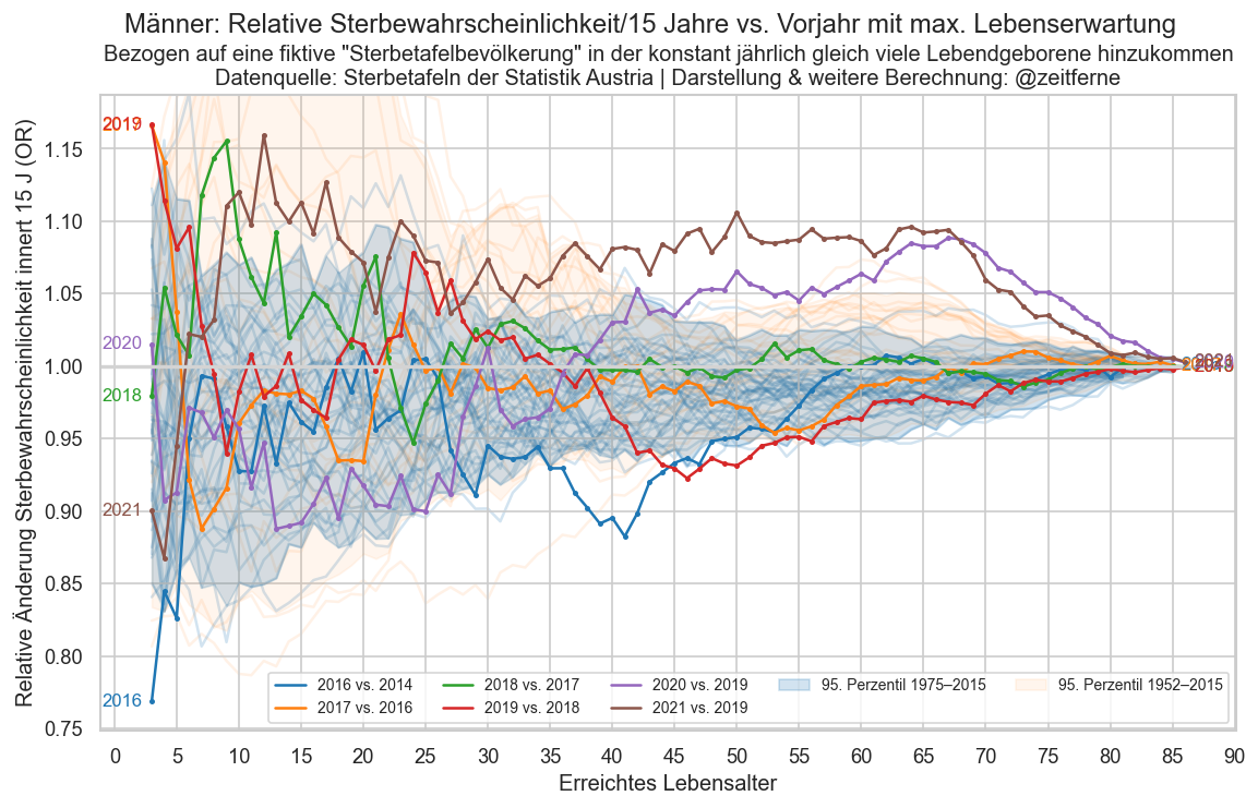
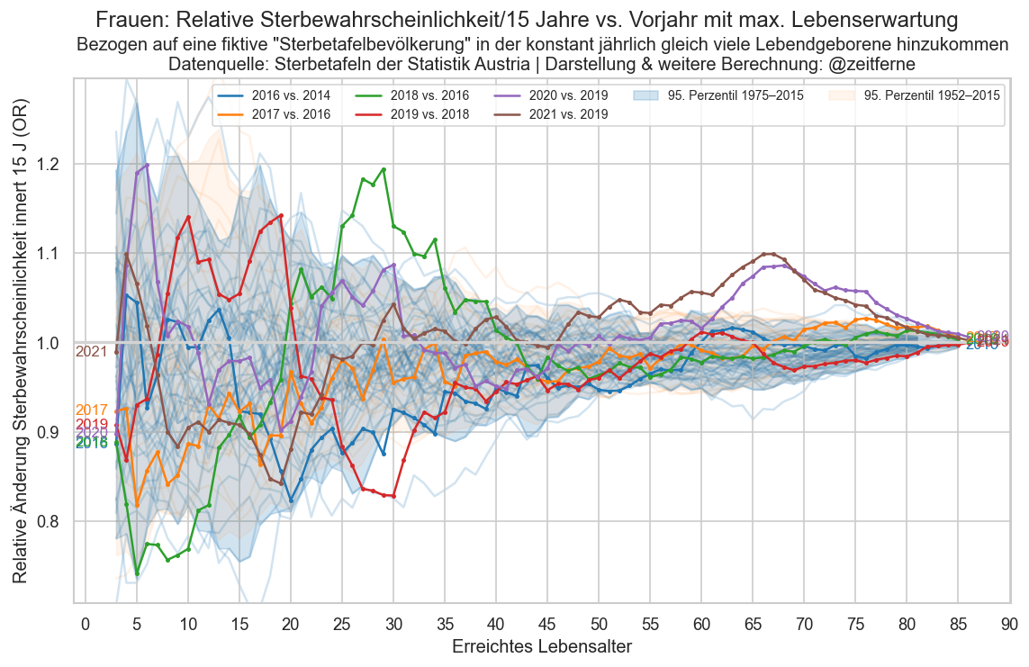
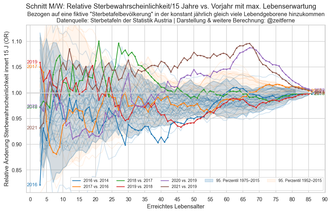
fig.suptitle(
f"{sexlabel(sex)}:"
f" {mainlabel} vs. Vorjahr mit max. Lebenserwartung")
ax.set_title(
"Bezogen auf eine fiktive \"Sterbetafelbevölkerung\" in"
" der konstant jährlich gleich viele Lebendgeborene hinzukommen"
"\nDatenquelle: Sterbetafeln der Statistik Austria | Darstellung & weitere Berechnung: @zeitferne")
return fig, ax
#ax.set_xlim(left=-1, right=50)
#ax.set_ylim(top=1.5)
#display(ststat.xs("m", level="sex").xs(38, level="age"))
#display(data.query("age == 63"))
In [17]:
maxrem = (
    ststat
    .xs(1, level="age")
    ["life_rem"]
    .groupby(level="sex")
    .transform(lambda g: g.rolling(5).agg(lambda s: s.idxmax()[0]).shift())
    .dropna()
    .astype(int)
).rename("maxrem_idx")

def join_maxrem(df):
    return (df
            .join(maxrem)
            .merge(
                df,
                left_on=["maxrem_idx", "sex", "age"],
                right_index=True,
                suffixes=(None, '_max')))
In [18]:
n_die_s = (
    ststat["n_die"]
    .groupby(["year", "sex"])
    .rolling(pd.api.indexers.FixedForwardWindowIndexer(window_size=15))
    .sum()
    .reset_index([0, 1], drop=True)#.query("age <= 95")["n_at"].copy()
)
p_die_s = (n_die_s / ststat["n_surv"]).rename("p_die_s")
#n_at.loc[n_at.index.get_level_values("age") == 95] = ststat["n_from"]
p_die_s_or = p_die_s / join_maxrem(p_die_s.to_frame())["p_die_s_max"]

def plt_die_or(sex):
    fig, ax = plt_year_comp(p_die_s_or, sex, "Relative Sterbewahrscheinlichkeit/15 Jahre")
    ax.set_ylabel("Relative Änderung Sterbewahrscheinlichkeit innert 15 J (OR)")
    ax.set_xlabel("Erreichtes Lebensalter")

for sex in ("m", "f", "amf"):
    plt.figure()
    plt_die_or(sex)
In [19]:
ststat.reset_index()["year"].min()
Out[19]:
1947
In [20]:
ststat.query("year == 2021")
Out[20]:
| life_rem | n_at | n_die | n_from | n_surv | p_die | life_sum | |||
|---|---|---|---|---|---|---|---|---|---|
| year | sex | age | |||||||
| 2021 | amf | 0 | 81.2814 | 99749.4145 | 273.0846 | 8.1281e+06 | 100000.0000 | 2.7308e-03 | 81.2814 |
| 1 | 80.5038 | 99718.1465 | 17.5379 | 8.0284e+06 | 99726.9154 | 1.7586e-04 | 81.5038 | ||
| 2 | 79.5178 | 99701.9134 | 14.9283 | 7.9287e+06 | 99709.3775 | 1.4972e-04 | 81.5178 | ||
| 3 | 78.5295 | 99689.4339 | 10.0306 | 7.8290e+06 | 99694.4492 | 1.0062e-04 | 81.5295 | ||
| 4 | 77.5373 | 99679.9620 | 8.9132 | 7.7293e+06 | 99684.4186 | 8.9413e-05 | 81.5373 | ||
| 5 | 76.5442 | 99669.8619 | 11.2870 | 7.6296e+06 | 99675.5054 | 1.1324e-04 | 81.5442 | ||
| 6 | 75.5529 | 99661.9090 | 4.6188 | 7.5299e+06 | 99664.2184 | 4.6343e-05 | 81.5529 | ||
| 7 | 74.5564 | 99656.6805 | 5.8382 | 7.4303e+06 | 99659.5996 | 5.8581e-05 | 81.5564 | ||
| 8 | 73.5607 | 99652.0084 | 3.5059 | 7.3306e+06 | 99653.7613 | 3.5182e-05 | 81.5607 | ||
| 9 | 72.5633 | 99648.4775 | 3.5557 | 7.2310e+06 | 99650.2554 | 3.5681e-05 | 81.5633 | ||
| 10 | 71.5659 | 99644.9638 | 3.4719 | 7.1313e+06 | 99646.6997 | 3.4842e-05 | 81.5659 | ||
| 11 | 70.5683 | 99641.4281 | 3.5994 | 7.0317e+06 | 99643.2278 | 3.6121e-05 | 81.5683 | ||
| 12 | 69.5709 | 99634.9152 | 9.4265 | 6.9320e+06 | 99639.6284 | 9.4606e-05 | 81.5709 | ||
| 13 | 68.5774 | 99627.2473 | 5.9094 | 6.8324e+06 | 99630.2020 | 5.9313e-05 | 81.5774 | ||
| 14 | 67.5815 | 99618.4795 | 11.6262 | 6.7328e+06 | 99624.2926 | 1.1670e-04 | 81.5815 | ||
| 15 | 66.5892 | 99596.5112 | 32.3103 | 6.6331e+06 | 99612.6663 | 3.2437e-04 | 81.5892 | ||
| 16 | 65.6104 | 99571.8656 | 16.9809 | 6.5335e+06 | 99580.3561 | 1.7055e-04 | 81.6104 | ||
| 17 | 64.6213 | 99547.8922 | 30.9660 | 6.4340e+06 | 99563.3752 | 3.1104e-04 | 81.6213 | ||
| 18 | 63.6411 | 99515.5752 | 33.6679 | 6.3344e+06 | 99532.4092 | 3.3830e-04 | 81.6411 | ||
| 19 | 62.6623 | 99481.6478 | 34.1869 | 6.2349e+06 | 99498.7412 | 3.4367e-04 | 81.6623 | ||
| ... | ... | ... | ... | ... | ... | ... | ... | ... | |
| mf | 81 | 8.4412 | 59520.6970 | 2983.0043 | 5.1502e+05 | 61012.1991 | 4.8892e-02 | 89.4412 | |
| 82 | 7.8494 | 56430.1489 | 3198.0918 | 4.5550e+05 | 58029.1948 | 5.5112e-02 | 89.8494 | ||
| 83 | 7.2781 | 53163.7182 | 3334.7696 | 3.9907e+05 | 54831.1030 | 6.0819e-02 | 90.2781 | ||
| 84 | 6.7170 | 49684.0858 | 3624.4952 | 3.4590e+05 | 51496.3334 | 7.0384e-02 | 90.7170 | ||
| 85 | 6.1877 | 45877.7131 | 3988.2503 | 2.9622e+05 | 47871.8382 | 8.3311e-02 | 91.1877 | ||
| 86 | 5.7047 | 41759.9502 | 4247.2755 | 2.5034e+05 | 43883.5879 | 9.6785e-02 | 91.7047 | ||
| 87 | 5.2624 | 37546.3470 | 4179.9309 | 2.0858e+05 | 39636.3124 | 1.0546e-01 | 92.2624 | ||
| 88 | 4.8238 | 33246.9648 | 4418.8335 | 1.7103e+05 | 35456.3816 | 1.2463e-01 | 92.8238 | ||
| 89 | 4.4394 | 28874.1048 | 4326.8865 | 1.3779e+05 | 31037.5481 | 1.3941e-01 | 93.4394 | ||
| 90 | 4.0775 | 24627.1115 | 4167.1003 | 1.0891e+05 | 26710.6616 | 1.5601e-01 | 94.0775 | ||
| 91 | 3.7388 | 20552.0259 | 3983.0707 | 8.4286e+04 | 22543.5613 | 1.7668e-01 | 94.7388 | ||
| 92 | 3.4339 | 16670.1398 | 3780.7017 | 6.3734e+04 | 18560.4906 | 2.0370e-01 | 95.4339 | ||
| 93 | 3.1843 | 13174.3496 | 3210.8787 | 4.7064e+04 | 14779.7889 | 2.1725e-01 | 96.1843 | ||
| 94 | 2.9294 | 10173.7438 | 2790.3329 | 3.3890e+04 | 11568.9103 | 2.4119e-01 | 96.9294 | ||
| 95 | 2.7016 | 7620.4562 | 2316.2423 | 2.3716e+04 | 8778.5773 | 2.6385e-01 | 97.7016 | ||
| 96 | 2.4906 | 5495.8897 | 1932.8908 | 1.6095e+04 | 6462.3351 | 2.9910e-01 | 98.4906 | ||
| 97 | 2.3401 | 3809.1021 | 1440.6842 | 1.0599e+04 | 4529.4442 | 3.1807e-01 | 99.3401 | ||
| 98 | 2.1984 | 2555.2932 | 1066.9336 | 6.7904e+03 | 3088.7600 | 3.4542e-01 | 100.1984 | ||
| 99 | 2.0947 | 1666.2241 | 711.2046 | 4.2351e+03 | 2021.8264 | 3.5176e-01 | 101.0947 | ||
| 100 | 1.9600 | NaN | 532.7704 | 2.5688e+03 | 1310.6218 | 4.0650e-01 | 101.9600 |
404 rows × 7 columns
In [21]:
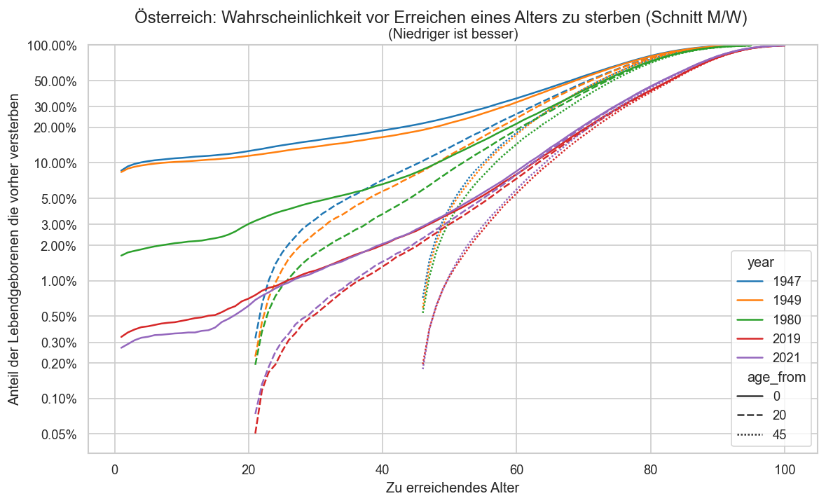
pdata = ststat.query("year in (1947, 1949, 1980, 2021, 2019) and sex == 'm'").copy()
#display(pdata)
#pal = sns.color_palette("plasma_r", n_colors=pdata["year"].nunique())
pal = sns.color_palette(n_colors=5) #["violet", "pink"] + sns.color_palette("Blues", 2) + sns.color_palette("Reds", 2)
pdata["pdie"] = 1 - pdata["n_surv"] / pdata.xs(0, level="age")["n_surv"]
pdata["age_from"] = 0
pdata_y = pdata.copy()
pdata_y["pdie"] = 1 - pdata_y["n_surv"] / pdata_y.xs(20, level="age")["n_surv"]
pdata_y["age_from"] = 20
pdata_y.set_index("age_from", append=True, inplace=True)
pdata_y = pdata_y.query("age > age_from")

pdata_y2 = pdata.copy()
pdata_y2["pdie"] = 1 - pdata_y2["n_surv"] / pdata_y2.xs(45, level="age")["n_surv"]
pdata_y2["age_from"] = 45
pdata_y2.set_index("age_from", append=True, inplace=True)
pdata_y2 = pdata_y2.query("age > age_from")
pdata.set_index("age_from", append=True, inplace=True)
pdata = pdata.query("age > 0")
pdata = pd.concat([pdata, pdata_y, pdata_y2])

pdata.reset_index(inplace=True)
ax = sns.lineplot(
    pdata,
    x="age", y="pdie", hue="year", style="age_from",
    palette=pal)
fig = ax.figure
#cov.labelend2(ax, pdata, "life_sum", cats="year", x="age", shorten=lambda y: y, colorize=pal, ends=(True, True))
#ax.legend(ncol=2)
ax.set_ylabel("Anteil der Lebendgeborenen die vorher versterben")
ax.set_title("(Niedriger ist besser)")
ax.set_xlabel("Zu erreichendes Alter")
#ax.set_ylim(bottom=81)
#ax.set_ylim(bottom=0)
cov.set_logscale(ax)
ax.set_ylim(top=1)
cov.set_percent_opts(ax, decimals=2)
#ax.set_ylim(bottom=0.01)

fig.suptitle("Österreich: Wahrscheinlichkeit vor Erreichen eines Alters zu sterben (Schnitt M/W)", y=0.95)
#ax.set_title("(Y-Achse beginnt nicht bei 0!)")
Out[21]:
Text(0.5, 0.95, 'Österreich: Wahrscheinlichkeit vor Erreichen eines Alters zu sterben (Schnitt M/W)')
In [22]:
ststat.query("sex == 'mf'").reset_index()["year"].unique()
Out[22]:
array([2002, 2003, 2004, 2005, 2006, 2007, 2008, 2009, 2010, 2011, 2012,
       2013, 2014, 2015, 2016, 2017, 2018, 2019, 2020, 2021], dtype=int64)
In [23]:
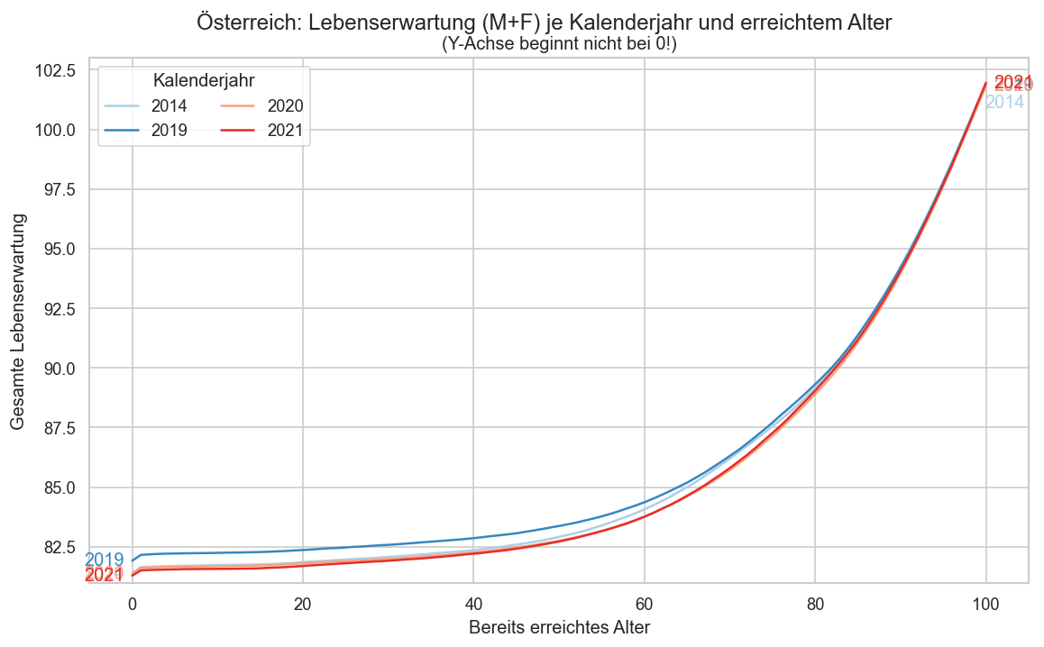
pdata = ststat.query("year in (2021, 2020, 2019, 2014) and sex == 'mf'").reset_index()
#pal = sns.color_palette("plasma_r", n_colors=pdata["year"].nunique())
pal = sns.color_palette("Blues", 2) + sns.color_palette("Reds", 2)
ax = sns.lineplot(
    pdata,
    x="age", y="life_sum", hue="year",
    palette=pal)
fig = ax.figure
#cov.set_logscale(ax)
cov.labelend2(ax, pdata, "life_sum", cats="year", x="age", shorten=lambda y: y, colorize=pal, ends=(True, True))
ax.legend(ncol=2, title="Kalenderjahr")
ax.set_ylabel("Gesamte Lebenserwartung")
ax.set_xlabel("Bereits erreichtes Alter")
ax.set_ylim(bottom=81)
fig.suptitle("Österreich: Lebenserwartung (M+F) je Kalenderjahr und erreichtem Alter", y=0.95)
ax.set_title("(Y-Achse beginnt nicht bei 0!)")
Out[23]:
Text(0.5, 1.0, '(Y-Achse beginnt nicht bei 0!)')
In [24]:
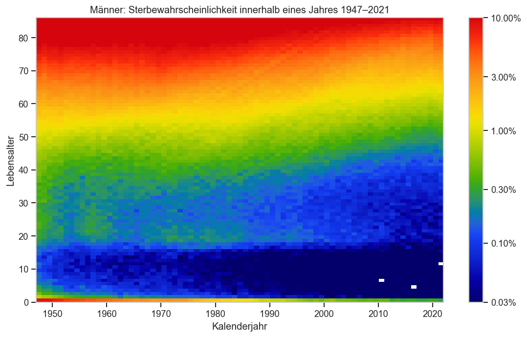
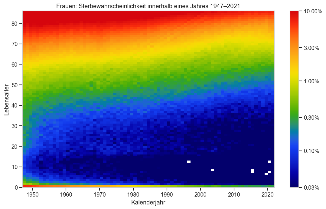
def plt_p_die_cmap(sex):
    fig, ax = plt.subplots()
    pdata = ststat.xs(sex, level="sex").query("age <= 85").reset_index().pivot(index="age", columns="year", values="p_die")
    #pdata = pdata / pdata.shift(axis="columns")
    im = ax.imshow(
        pdata,
        cmap=cov.un_cmap,
        interpolation='none',
        origin="lower", aspect="auto",
        extent=[
            pdata.columns[0],
            pdata.columns[-1] + 1,
            pdata.index[0],
            pdata.index[-1] + 1,
        ],
        #norm=matplotlib.colors.TwoSlopeNorm(vmin=0.75, vcenter=1, vmax=1.1),
        norm=matplotlib.colors.LogNorm(vmin=0.0003, vmax=0.1)
    )
    ax.grid(False)
    cax = fig.colorbar(im)
    cov.set_logscale(cax.ax, reduced=True)
    cov.set_percent_opts(cax.ax, decimals=2)
    ax.set_ylabel("Lebensalter")
    ax.set_xlabel("Kalenderjahr")
    ax.set_title(sexlabel(sex) + ": Sterbewahrscheinlichkeit innerhalb eines Jahres" +
                 f" {pdata.columns[0]}‒{pdata.columns[-1]}")
    ax.tick_params(left=True, bottom=True)

plt_p_die_cmap("m")
plt_p_die_cmap("f")
In [25]:
st.index.get_level_values("sex").unique()
---------------------------------------------------------------------------
NameError                                 Traceback (most recent call last)
Cell In[25], line 1
----> 1 st.index.get_level_values("sex").unique()

NameError: name 'st' is not defined
In [26]:
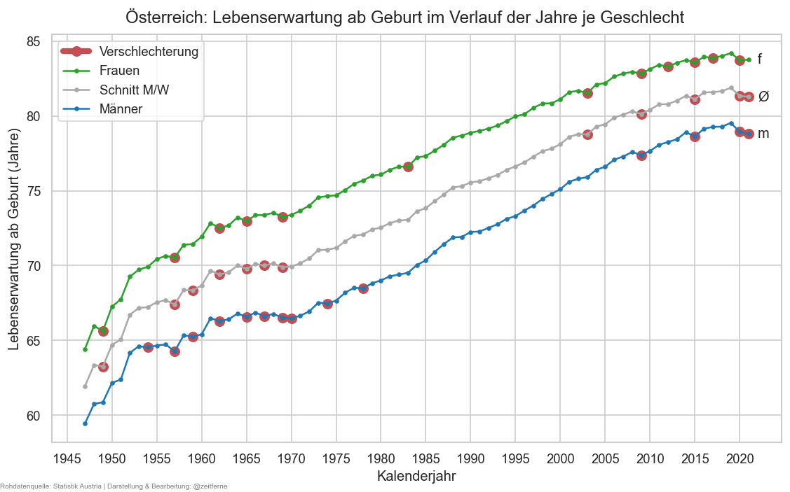
def plt_lexp():
    stat0 = ststat.xs(0, level="age")#.query("year >= 2000")
    fig, ax = plt.subplots()
    cats = [("m", "C0"), ("amf", "darkgrey"), ("f", "C2")]
    cats.reverse()
    for sex, cl in cats:
        stat0x = stat0.xs(sex, level="sex")["life_sum"]
        is_worsened = stat0x < stat0x.shift()
        ax.plot(stat0x.where(is_worsened), marker="o", color="r", markersize=8, lw=5,# alpha=0.7,
                label="Verschlechterung" if sex is cats[0][0] else None)
        ax.plot(stat0x, marker=".", label=sexlabel(sex), color=cl)
        ax.annotate(r"Ø" if sex == "amf" else sex,
                    (stat0x.index[-1] + 1, stat0x.iloc[-1]), va="center")
    fig.suptitle(f"Österreich: Lebenserwartung ab Geburt im Verlauf der Jahre je Geschlecht", y=0.93)
    ax.legend()
    #cov.set_percent_opts(ax)
    ax.xaxis.set_major_locator(matplotlib.ticker.MultipleLocator(5))
    ax.set_xlabel("Kalenderjahr")
    ax.set_ylabel("Lebenserwartung ab Geburt (Jahre)")
    stampit(fig)
plt_lexp()
In [27]:
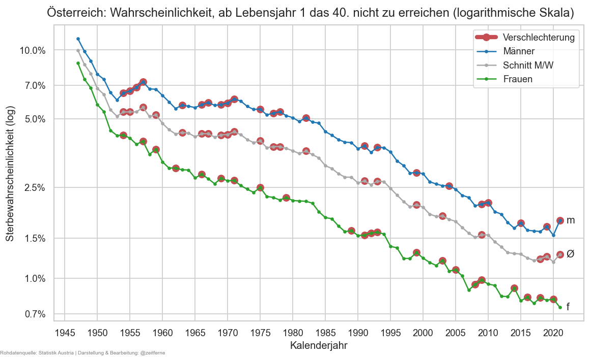
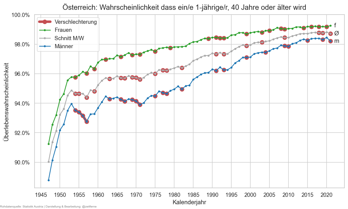
def plt_die50(relative=False):
    stat0 = ststat#.xs("f", level="sex")#.query("year >= 2000")
    tgtage = 40
    fromage = 1
    nsurv50 = stat0.xs(tgtage, level='age')["n_surv"]
    psurv50 = nsurv50 / stat0.xs(fromage, level='age')["n_surv"].rename("p_surv_rng")
    if relative:
        psurv50 = 1 - psurv50
    fig, ax = plt.subplots()
    cats = [("m", "C0"), ("amf", "darkgrey"), ("f", "C2")]
    if not relative:
        cats.reverse()
    for sex, cl in cats:
        psurv50x = psurv50.xs(sex, level="sex")
        if relative:
            is_worsened = psurv50x > psurv50x.shift()
        else:
            is_worsened = psurv50x < psurv50x.shift()
        ax.plot(psurv50x.where(is_worsened), marker="o", color="r", markersize=8, lw=5,# alpha=0.7,
                label="Verschlechterung" if sex is cats[0][0] else None)
        ax.plot(psurv50x, marker=".", label=sexlabel(sex), color=cl)
        ax.annotate(r"Ø" if sex == "amf" else sex,
                    (psurv50x.index[-1] + 1, psurv50x.iloc[-1]), va="center")
    if relative:
        cov.set_logscale(ax)
        ax.yaxis.set_major_locator(matplotlib.ticker.LogLocator(
            base=10, subs=[0.15, 0.25, 0.5, 0.7, 1]
        ))
    else:
        ax.set_ylim(top=1)
    fig.suptitle(
        f"Österreich: Wahrscheinlichkeit, ab Lebensjahr {fromage} das {tgtage}. nicht zu erreichen (logarithmische Skala)" if relative else
        f"Österreich: Wahrscheinlichkeit dass ein/e {fromage}-jährige/r, {tgtage} Jahre oder älter wird",
        y=0.93)
    ax.legend()
    cov.set_percent_opts(ax, decimals=1 if psurv50.min() < 0.01 or psurv50.max() > 0.99 or psurv50.min() < 3 and relative else 0)
    ax.xaxis.set_major_locator(matplotlib.ticker.MultipleLocator(5))
    ax.set_xlabel("Kalenderjahr")
    ax.set_ylabel("Sterbewahrscheinlichkeit (log)" if relative else "Überlebenswahrscheinlichkeit")
    stampit(fig)
plt_die50(True)
plt_die50(False)